The Simplest Circuit
The key idea for this section is that steady-state expression levels depend on protein production and removal rates.
Let’s break that down.
First, steady-state conditions mean that all inputs to the system are constant forever. That simplifies things quite a bit.
Expression levels are just the net amount of proteins produced.
So, how many proteins there are, with no variables, depends on how many proteins are being created and how many are being removed. Simple, right?
Now, the circuit. This circuit is the simplest possible circuit: a single gene — let’s call it \(x\) — coding for a single protein \(p\) at a rate of \(\beta\) molecules per unit time.
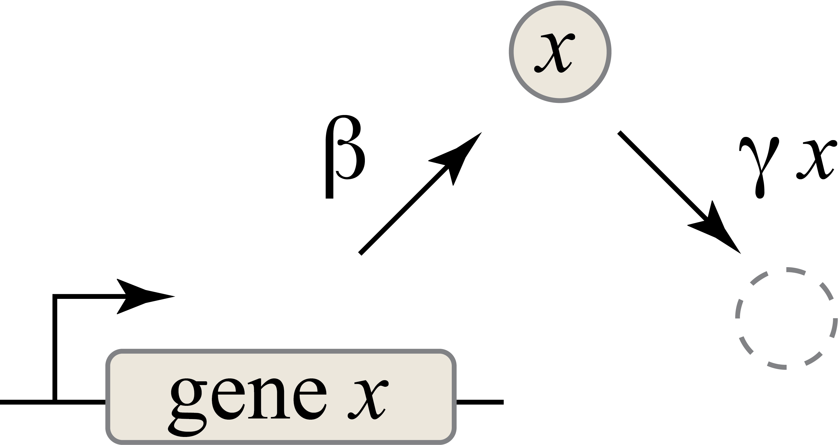 Credit: CalTech
However, in real life, proteins aren’t just made forever; they’re also reduced, through both active degradation (being broken down) and dilution (the cell getting bigger, which reduces the protein’s concentration). That’s represented above by the dashed circle. For simplicity, let’s say that it’s being reduced at a rate constant \(\gamma\) (that letter is a gamma, for anyone who wanted to know). Note that this is not just a rate — it’s a rate constant, meaning that the actual rate is proportional to the number of molecules. More molecules, more reduction.
There’s a differential equation for this: \(\frac{dx}{dt} = \text{production} - (\text{degradation} + \text{dilution})\)
Or: \(\frac{dx}{dt} = \beta - \gamma x\)
Since \(\gamma\) counts both degradation and dilution, we can say that: \(\gamma = \gamma_\text{degradation} + \gamma_\text{dilution}\)
Since we’re getting into the math, a quick tip: if you (like me) forget what a variable does halfway through the page, just hover over it and it’ll tell you what it does. Because of the way it’s rendered, it might not work in some cases, but feel free to try it. Anyway, back to the show.
To find the net production of the protein under steady state conditions, set the derivative to zero and solve for \(x\):
\[0 = \beta - \gamma x\] \[-\beta = -\gamma x\] \[\frac{-\beta}{-\gamma} = x\] \[\frac\beta\gamma = x\]And we find that steady-state protein concentration is proportional to the ratio of production and removal rates. This is another core concept that should be built as intuition.
Since I haven’t used the interactive graphing functions I took the bandwidth to import yet, let’s graph the general shape of the protein concentration function under the simplest possible conditions (play with the sliders!):
\[f(t)=xt=\frac{\beta t}{\gamma}\]It’s a line — for now.
Considering Transcription
Right now, we have protein synthesis as one process — no intermediate steps. In reality, it has two: transcription and translation. The mRNA made in transcription can also be degraded and diluted, just like the proteins made in translation. Let’s add another variable to represent mRNA — call it \(m\). This can be shown in a diagram:
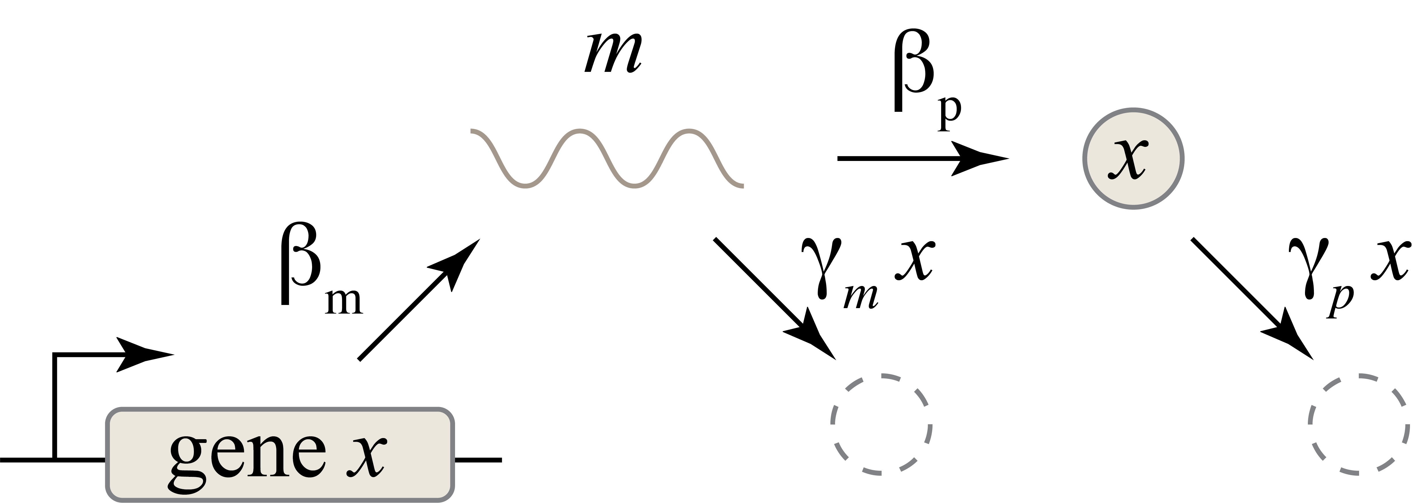 Credit: CalTech
The reaction can now be described by two coupled differential equations:
\[\frac{dm}{dt} = \beta_m - \gamma_mm\] \[\frac{dx}{dt} = \beta_pm - \gamma_px\]Now, to find steady-state mRNA and protein concentrations, we set both derivatives to zero and solve, giving us:
\[m_{ss}=\frac{\beta_m}{\gamma_m}\] \[x_{ss}=\frac{\beta_pm_{ss}}{\gamma_p}=\frac{\beta_p\beta_m}{\gamma_p\gamma_m}\]This tells us that steady-state protein concentration, when we consider transcription and translation as separate steps, is proportional to the product of the two synthesis rates and inversely proportional to the product of the two degradation rates. Again, if you think about it, that’s pretty intuitive.
Here’s a graph to play with:
It’s still a line. Onwards!